Image and Text Contrast Detection

By Capital Technology Group's Fall 2022 Data Science intern, Akiva Neuman.
The Web Content Accessibility Guidelines (WCAG) are a list of recommendations for making web content more accessible for people with disabilities as well as for all users. The WCAG states that the contrast requirement for text visibility in an image to be sufficient is 4.5:1.


I began this project with the task of determining firstly how to tell whether there was text in an image and then whether the text had adequate contrast with the rest of the image for a person including people who have visual impairment. I decided to attempt to solve the problem using convolutional neural networks(CNNs), one, trained on text and no text images, to determine whether there was text in an image and then if there is text the image would be passed onto another CNN that would be trained on high and low contrast images to determine whether the image to text contrast ratio is sufficient. I built a function that used the googlesearch module to find websites that had images with text in them and then the beautiful soup module to web scrape the images from the sites. Using this function, I entered the search “images with text in them” and collected 3000 images with text in them and also collected another 3000 images without text in them. Afterward, I went through the collected data myself to make certain that it was clean data by including mislabeled text images into the text image class and mislabeled nontext images into the nontext image class.
The next step was to model the data. The data images need to first be preprocessed because the features of the image, for example, size and pixel range, need to be uniform for the model to train well on the data. Using Tensorflow, I preprocessed the image with an image generator, normalizing the images to convert the pixels in range 0 to 255 to be in the range 0 to 1, making the images 256 by 256, and then creating a train, validation, and test set. I used 20% of the data for validation and 8% for testing. A convolutional neural network has a series of convolutional and pooling layers that are used to dissect an image to find patterns in the pixel data. I built the model having three convolutional layers each followed by a max pooling layer. The convolutional layers use filter matrices to pass over the image and take the dot product of the filter and the part of the matrix it’s passing, then the max pooling layer takes the maximum value from the resulting matrix, which is then passed onto the next layer.
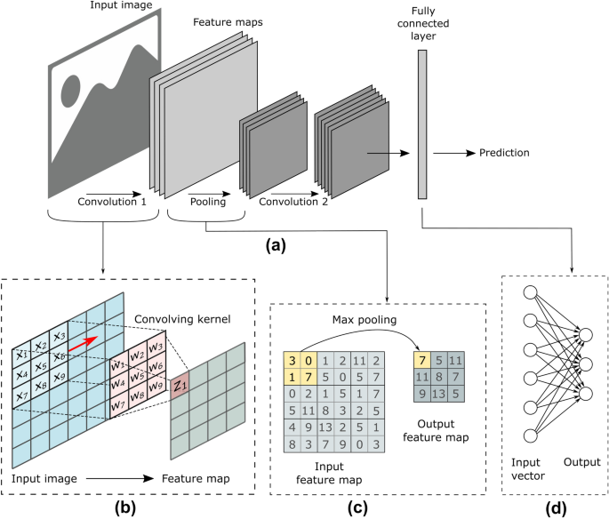
This process generalizes the image to abstract patterns that wouldn’t otherwise be apparent. Afterward, the result is flattened to one dimension and then passed through a dense layer, which is a compilation of layers of neurons with weight and bias linear functions where, as opposed to a convolutional layer, all input nodes affect all output nodes. The weight and bias linear function is passed through an activation function before being passed to the next layer. Activation functions are used to introduce nonlinearity to the model, which allows the model to better fit the data, and ultimately decide whether the neuron should be activated to pass data to the next layer. There are regularization techniques like dropout that automatically deactivate random neurons to decrease the likelihood of overfitting. The vanishing gradient problem is a phenomenon where the gradient updates within the activation function, which are calculated from the optimization of a cost function, tend toward 0 making the weights ineffective. Therefore, using an effective activation function is critical. The convolutional layers used the activation function leaky ReLU and the final layer used sigmoid. I chose leaky ReLU because ReLU by itself is very powerful in how it treats negative values becoming 0 and positive value derivatives being 1 to solve the vanishing gradient problem by backpropagating only if the value is 1, but changing the negative weight values to 0 I preferred not to do and instead to use leaky ReLU to give the negative weights some flexibility.
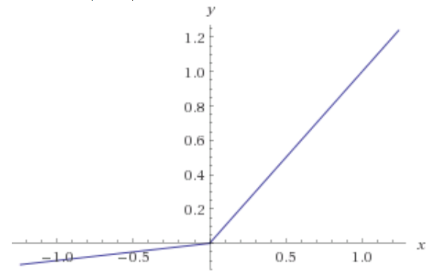
Sigmoid was used to return a value of 0 or 1.
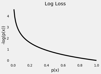
A loss function is used to optimize it with respect to the weights and biases, thus reducing the loss function to its minima, which reduces the error of the model. An optimization function is used to increase convergence to the minima. Metrics are used to evaluate model performance. I compiled the model with binary cross entropy loss function because my dependent variable is binary, adam optimization because it has the fastest computation time, and metrics of accuracy, precision, recall, and f1 to measure model performance. The cost function binary cross entropy takes the negative log-likelihood of all the positive (1) and negative (0) cases and when the observation is positive the part of the formula after the plus sign disappears and the part before the plus sign disappears when the observation is negative,
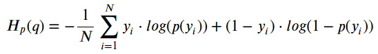
thus penalizing incorrect predictions because log loss increases exponentially as p(x) approaches 0.
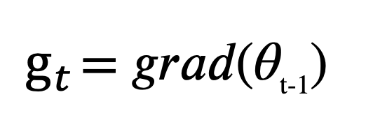
For optimizers, adam generally has the quickest computation time to convergence by taking the derivative of the cost function with respect to the parameters,
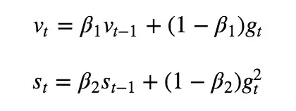
and then updates the gradients for the first and second moment, the larger beta is, the more gradient steps are calculated,
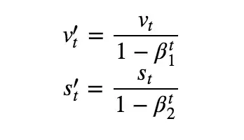
by then computing the biased corrected moments,
and then updating the parameters by multiplying the learning rate, which is updated individually for each weight, by the first corrected moment divided by the square root of the second corrected moment plus a small constant and then subtracting from the previous parameter to get the new parameter.
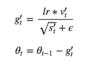
These moments are estimated from the exponentially moving average of the gradients and are used to increase convergence momentum toward the minima of the cost function.

There are four possibilities that a predicted value can have: true positive, true negative, false positive, or false negative.
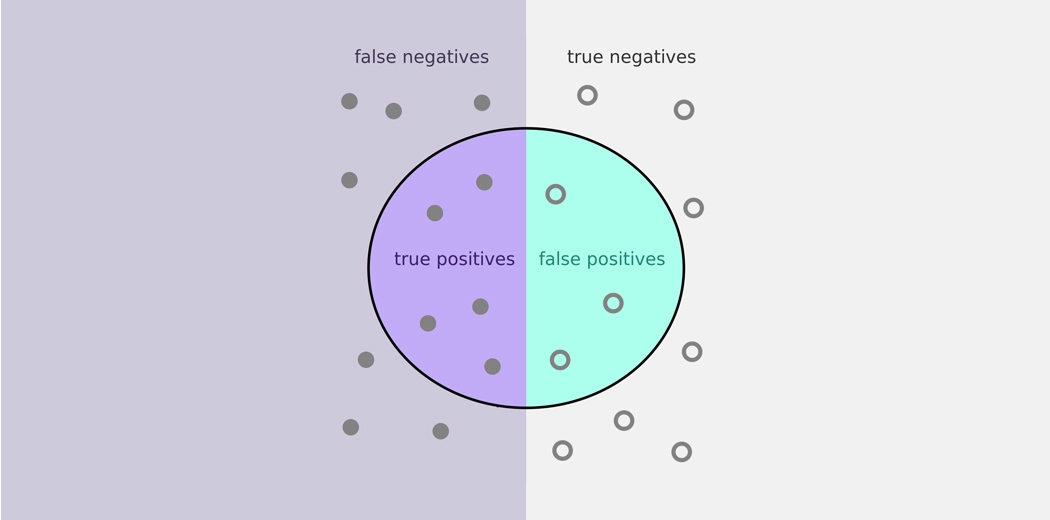
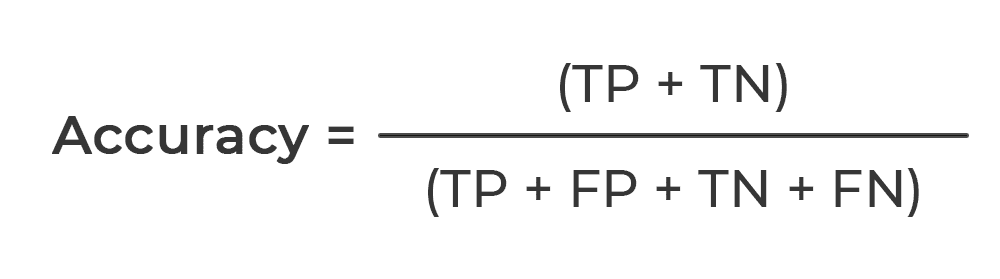
Accuracy is the true cases divided by the total cases.
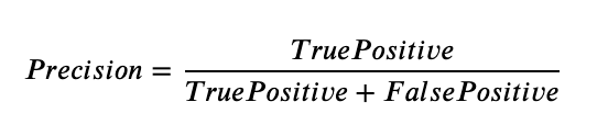
Precision is the true positives divided by the true positives plus the false positives.
Recall is the true positives divided by the true positives plus the false negatives.

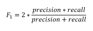
F1 is the harmonic mean of precision and recall.
The training and validation metrics for the model over 11 epochs were as follows:
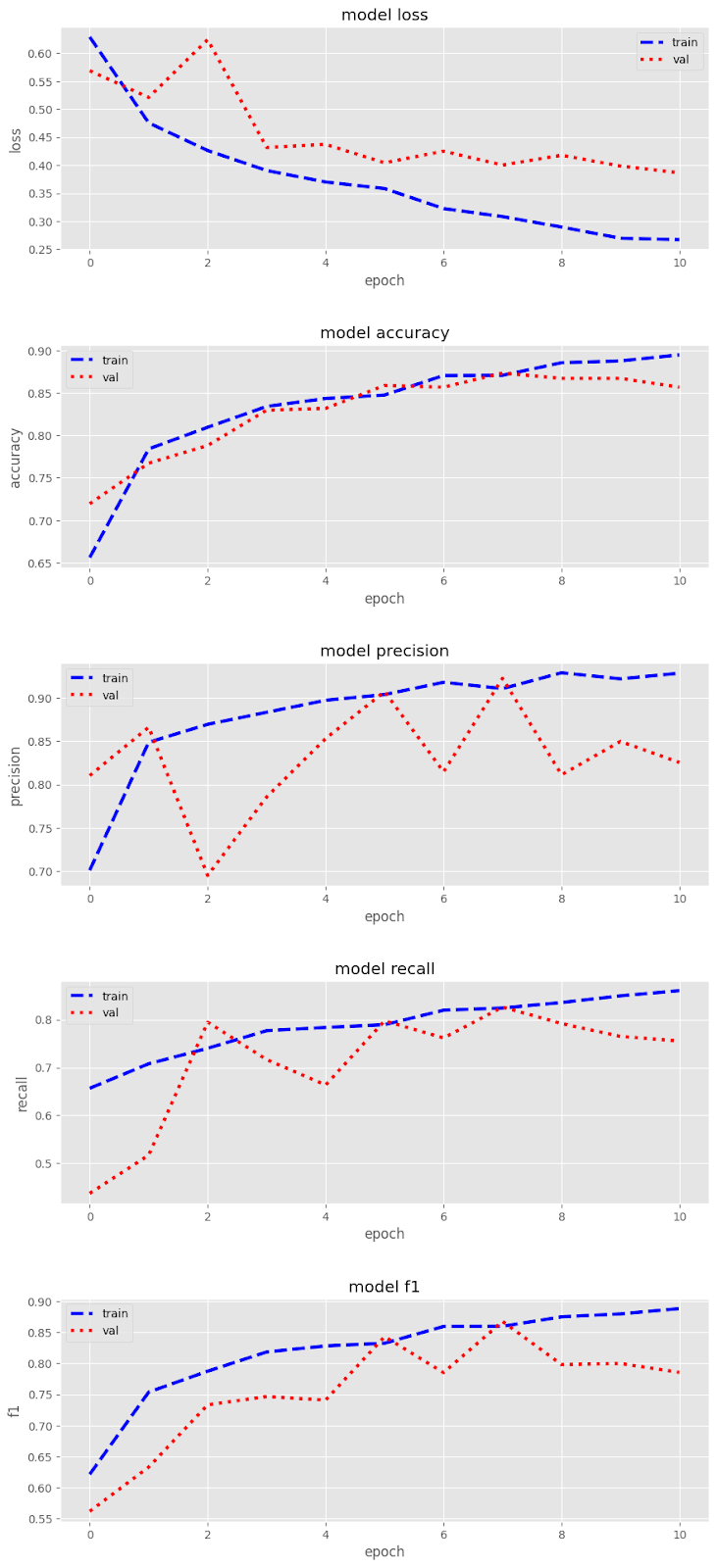
The test metrics:
Accuracy: 0.859
Precision: 0.882
Recall: 0.835
F1: 0.858
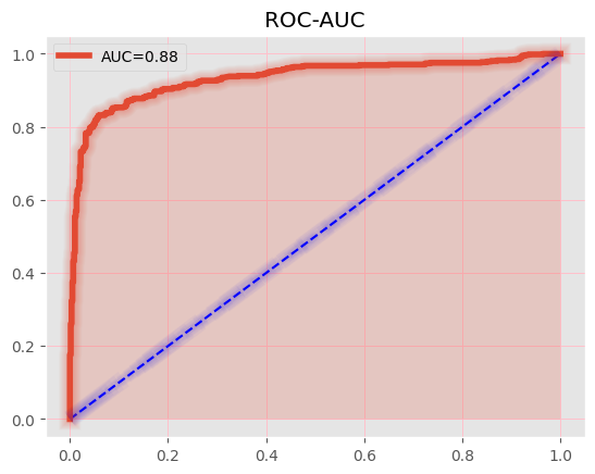
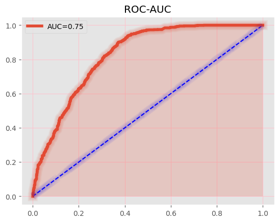
Receiver operating characteristic area under the curve(ROC AUC) is the true positive rate to false positive rate. The blue line is an average model.

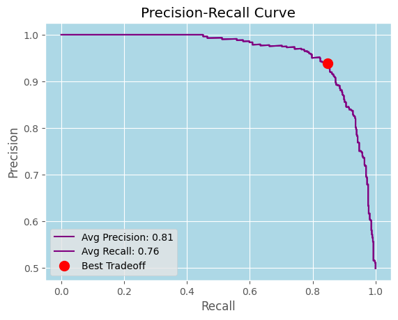
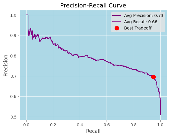
I didn’t use the "optimal" model precision recall tradeoff because I wanted the high precision to eliminate as many false positives as reasonably possible, but the following is the PRT graph.
The model tested well, but before I cross validated, I wanted to try to enhance the model with a random grid search of the hyperparameters based on validation loss using keras_tuner. I found a model that beat the previous model loss by 2 points.
The tuned model test metrics were as follows:
Accuracy: 0.881
Precision: 0.940
Recall: 0.820
F1: 0.876
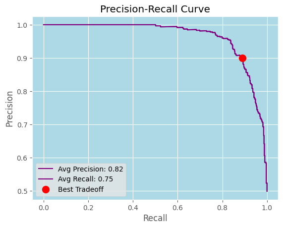
The higher precision without much recall expense was advantageous.
The tuned model cross-validated well with an accuracy score of .848.
I then used the pillow module on the existing images to create a second dataset that is half images with sufficient contrast and half with insufficient contrast. The next CNN needed some extra adjustments to be effective. Firstly, I used six convolutional and pooling layers to really go deep into the image to find the contrast feature. I also doubled my data from 6000 to 12000 images by cloning the images and then adjusting half of them using techniques like shear and zoom. Lastly, the model was originally favoring recall significantly, so I used the class weight hyperparameter to give negative cases more weight, thus increasing the model's false negatives, which in turn decreases the false positives and increases precision. The model training and validation metrics over 11 epochs were the following:
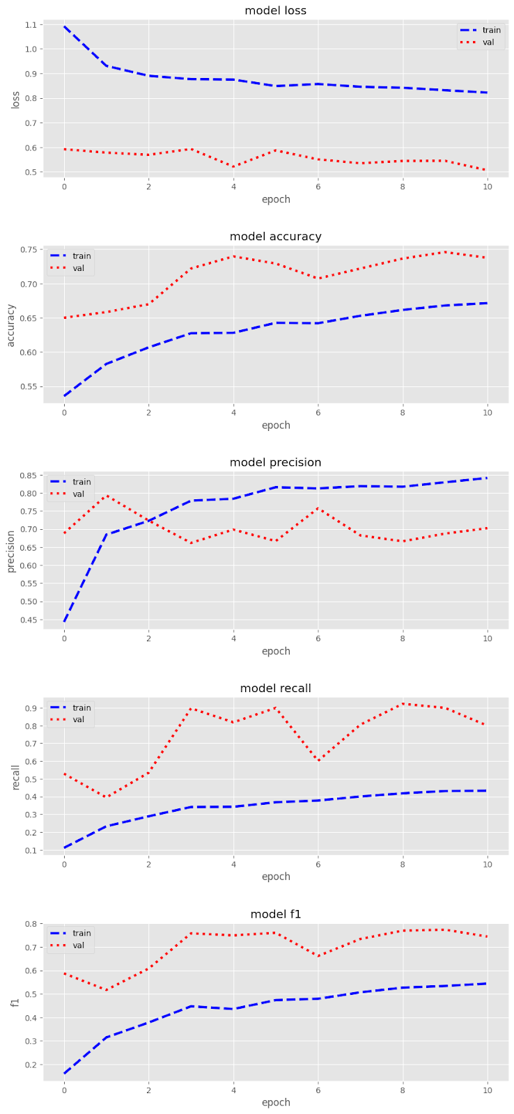
Notice that validation did better than training, but the model is not overfitting because it tested well. The following are the test metrics:
Accuracy: 0.754
Precision: 0.728
Recall: 0.824
F1: 0.773
The model also cross-validated well with an accuracy score of .724.
These models were built to favor precision because I want to remove as many false positives (images with no text or low contrast being classified otherwise). Recall was still above 80% for both models. The contrast model was having trouble classifying negative cases correctly, but by using the methods described, I was able to get precision above 70%. The models can now be used by developers to help automatically determine whether their content meets the contrast requirement of WCAG.